
Molecular Dynamics Background
Background
It is this simple, take a collection of particles and compute the interaction between all of them with each other in a system and predict how they will interact over time. This sounds very simple, but there is a whole lot of difficulty couched in the above problem. Fortunately for computational scientists, solving this problem touches a large range of different scientific disciplines. Fluid dynamics, cosmology, sociology, chemistry and particle physics the N-body interacting particle problem is pervasive and useful.Computation biologists have probably been the field to take this problem the furthest in their modeling of large molecular systems of interest as a collection of particles governed by classical potentials. The so-called Molecular Dynamics method is by far the most widely used computational method on today?s NSF computational resources, and is the driving algorithm behind programs such as NAMD, AMBER, DESMOND, and LAMMPS which are codes that have been scaled to 100,000s of cores on HPC architectures. At the heart each of these programs, is the integration of the particle positions over time expressed as a discrete iterative process where the forces of each particle in the system is computed at an instant in time and used to propagate their positions to the next timestep.
We will be working in this example on a fairly simple version of this algorithm where we will have a collection of random Argon atoms in a flat box, each with varying mass and positions. Space will be divided into ?cells? in which each particle will belong, which will allow us to neglect particles that have negligible contribution to the force of a particle. We will then update the particles positions and move onto the next timestep.
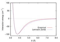
The particular potential we will be using in this example to govern the particles in the system is known as the Lennard-Jones potential, named after John Lennard-Jones who proposed it in 1924. It is also known at the 6-12 potential, and has the form:
This potential is fitted to reproduce quantum chemistry results. Figure 1 is a plot of the L-J potential for Argon as a function of the distance between two atoms. Normally, the L-J potential is defined specifically for types of atom.
For a discussion of Molecular Dynamics, see http://en.wikipedia.org/wiki/Molecular_dynamics
The Algorithm
We will be working with Argon atoms, there are several parameters that we will be fixing in our algorithm. These parameters will be fixed in the code for the purposes of our exercises.- We will be using 1.0 fs timestep, meaning that we will propogate 1 fs in time at every iteration.
- The mass of Argon is 39.849 a.u. and the density in 2 Dimension is 0.052 Atoms/Angstrom2
- Our cells dimensions will be 12 Angstroms (an Angstrom is a common unit of measurement in chemistry and is equivalent to 10-11 meters).
- No atom can begin the simulation less than 2 Angstroms apart, otherwise, the L-J potential will blow up.
- The L-J potential is defined for Argon as having ?=119.8 K and ? = 3.405 Angstroms. (see Figure 1 for what the potential looks like).
- Based on number of particles and the cutoff (in each cells, allocate space to hold the particles positions, and forces, indexed by cell.
- Begin loop over the cells in the system and compute the forces resulting from the potential of all of the particles that are in the same cell. Computing the force requires computing the derivative with respect to R of the potential.
- The loop over all of the cells to compute the forces resulting from the particles that reside in an adjacent cell.
- Once all of the forces have been calculated, use the forces to propagate the all of the particles in the system to their positions for the next times step.
- Iterate till completion.
Molecular Dynamics Exercise 1
Molecular Dynamics Exercise 2
Molecular Dynamics Exercise 3
Molecular Dynamics Exercise 4
Molecular Dynamics Exercise 5